Space Time Prediction - Re-balancing Bike Demands
John Paul Gitata
9/21/2022
1. Introduction
A bike share program is a shared transport service in which bicycles are made available for shared use to individuals on a short term basis for a price.
This project developed a method of predicting bike share trips in Manhattan Island, with emphasis on bike share demand. This document outlines the motivation for this project, exploratory analysis, feature engineering and model building.
1.2 Motivations
As the day progresses by there tends to be an unbalanced distribution of bikes in space. Bike share is not useful if a dock has no bikes to pick up, nor if there is no open docking space to deposit a bike.
Re-balancing is the practice of predicting bike share demand for all docks at all times and manually allocating bikes to docks with high demand.
1.3 Data Sources
To develop this model, I relied on three main datasets..
| Dataset | Source |
|---|---|
| Citibike Trips | NYC Department of Transportation |
| Apartments and Parks | OpenStreetMap |
| Demographics | NYC Census, Year 2018 |
1.4 Note
This project demands a lot of RAM, to handle the predictions.
2. Setup
2.1 Libraries
# change the colors add x y labs
library(tidyverse)
library(ggplot2)
library(sf)
library(tidycensus)
library(lubridate)
library(tigris)
library(osmdata)
library(gganimate)
library(riem)
library(FNN)
library(gridExtra)
library(grid)
library(knitr)
library(gifski)
library(rjson)
library(kableExtra)

options(tigris_class = "sf")
2.1 Themes and Functions
# Theme for our notebook
palette5 <- c("#f9b294","#f2727f","#c06c86","#6d5c7e","#315d7f")
palette4 <- c("#f9b294","#f2727f","#c06c86","#6d5c7e")
palette2 <- c("#f9b294","#f2727f")
palette1_main <- "#F2727F"
palette1_assist <- '#F9B294'

mapTheme <- function(base_size = 10, title_size = 18) {
theme(
text = element_text( color = "black"),
plot.title = element_text(hjust = 0.5, size = title_size, colour = "black",face = "bold"),
plot.subtitle = element_text(hjust = 0.5,size=base_size,face="italic"),
plot.caption = element_text(size=base_size,hjust=0),
axis.ticks = element_blank(),
panel.spacing = unit(6, 'lines'),
panel.background = element_blank(),
panel.grid.major = element_blank(),
panel.grid.minor = element_blank(),
panel.border = element_blank(),
strip.background = element_rect(fill = "grey80", color = "white"),
strip.text = element_text(size=base_size),
axis.title = element_text(face = "bold",size=base_size),
axis.text = element_blank(),
plot.background = element_blank(),
legend.background = element_blank(),
legend.title = element_text(size=base_size,colour = "black", face = "italic"),
legend.text = element_text(size=base_size,colour = "black", face = "italic"),
strip.text.x = element_text(size = base_size,face = "bold")
)
}

plotTheme <- function(base_size = 10, title_size = 18) {
theme(
text = element_text( color = "black"),
plot.title = element_text(hjust = 0.5, size = title_size, colour = "black",face = "bold"),
plot.subtitle = element_text(hjust = 0.5,size=base_size,face="italic"),
plot.caption = element_text(size=base_size,hjust=0),
axis.ticks = element_blank(),
panel.spacing = unit(6, 'lines'),
panel.background = element_blank(),
panel.grid.major = element_line("grey80", size = 0.1),
panel.grid.minor = element_blank(),
panel.border = element_rect(colour = "black", fill=NA, size=6),
strip.background = element_rect(fill = "grey80", color = "white"),
strip.text = element_text(size=base_size),
axis.title = element_text(face = "bold",size=base_size),
axis.text = element_text(size=base_size),
plot.background = element_blank(),
legend.background = element_blank(),
legend.title = element_text(size=base_size,colour = "black", face = "italic"),
legend.text = element_text(size=base_size,colour = "black", face = "italic"),
strip.text.x = element_text(size = base_size,face = "bold")
)
}

q5 <- function(variable) {as.factor(ntile(variable, 5))}

qBr <- function(df, variable, rnd) {
if (missing(rnd)) {
as.character(quantile(round(df[[variable]],0),
              c(.01,.2,.4,.6,.8), na.rm=T))
} else if (rnd == FALSE | rnd == F) {
as.character(formatC(quantile(df[[variable]],
                      c(.01,.2,.4,.6,.8), na.rm=T),
            digits = 3))
}
}

# Functions
nn_function <- function(measureFrom,measureTo,k) {
measureFrom_Matrix <- as.matrix(measureFrom)
measureTo_Matrix <- as.matrix(measureTo)
nn <-
get.knnx(measureTo, measureFrom, k)$nn.dist
output <-
as.data.frame(nn) %>%
rownames_to_column(var = "thisPoint") %>%
gather(points, point_distance, V1:ncol(.)) %>%
arrange(as.numeric(thisPoint)) %>%
group_by(thisPoint) %>%
summarize(pointDistance = mean(point_distance)) %>%
arrange(as.numeric(thisPoint)) %>%
dplyr::select(-thisPoint) %>%
pull()

return(output)
}
3. Data Wrangling
Reading in the bike data.
We also use the data to create bins of 60 minutes and weekly intervals.
trip1 <- read_csv('../input/tripdata/202205-citibike-tripdata.csv/202205-citibike-tripdata.csv')
trip2 <- read_csv('../input/tripdata/202206-citbike-tripdata.csv/202206-citbike-tripdata.csv')

trip_1 <- trip1 %>%
mutate(interval_hour = ymd_h(substr(started_at, 1, 13)),
week = week(interval_hour),
dayotw = wday(interval_hour, label = TRUE),
start_station_name = as.character(start_station_name),
end_station_name = as.character(end_station_name)) %>%
filter(week %in% c(18:22))

trip_2 <- trip2 %>%
mutate(interval_hour = ymd_h(substr(started_at, 1, 13)),
week = week(interval_hour),
dayotw = wday(interval_hour, label = TRUE),
start_station_name = as.character(start_station_name),
end_station_name = as.character(end_station_name)) %>%
filter(week %in% c(18:22))

bike_trip <- rbind(trip1, trip2)
glimpse(bike_trip)
3.1 Research Area
The research focus on Manhattan Island, the most densely populated and geographically smallest of the five areas of New York CIty. Manhattan has abundant transportation activities and Citi Bike share activities.
ride_rsch <- bike_trip %>%
group_by(start_station_name) %>%
summarize(lat = first(start_lat), lng=first(start_lng))

NYCTracts <-
tigris::tracts(state = "New York", county = "New York") %>%
dplyr::select(GEOID) %>%
filter(GEOID != "36061000100")

ride2_sf <- st_as_sf(ride_rsch, coords=c("lng", "lat"),
        crs = st_crs(NYCTracts), agr = "constant")

ride_station <- st_join(ride2_sf, NYCTracts, left = TRUE) %>% na.omit()
ride_tract <- st_join(NYCTracts, ride2_sf, left=TRUE) %>% na.omit()

station_list <- ride_station[["start_station_name"]]

ride3 <- bike_trip %>%
filter(start_station_name %in% station_list, end_station_name %in% station_list)

ggplot() +
geom_sf(data = st_union(NYCTracts), color = "black", size = 2) +
geom_sf(data = NYCTracts, color = "black", size = 0.1, linetype = "dashed", fill = "transparent") +
geom_sf(data =  ride_station, color = palette1_main, size = 0.5) +
labs(title = "Map of Manhattan Bike Ride Stations",
subtitle = "Red dots are bike stations") +
mapTheme()
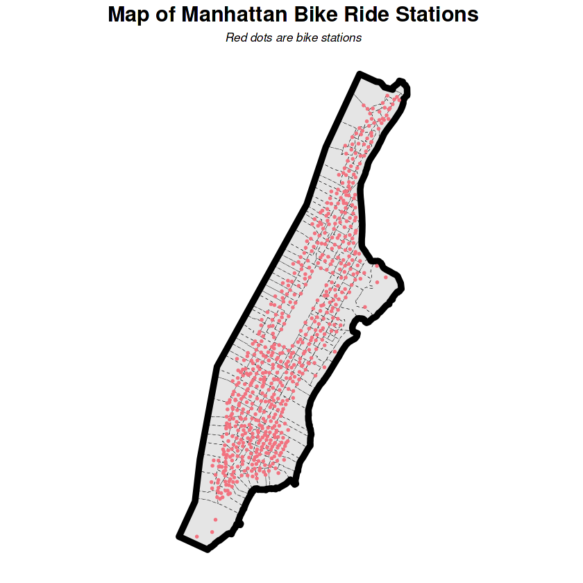
Re-balancing will happen among these bike share stations. The unit of analysis is the bike share station not the census tracts.
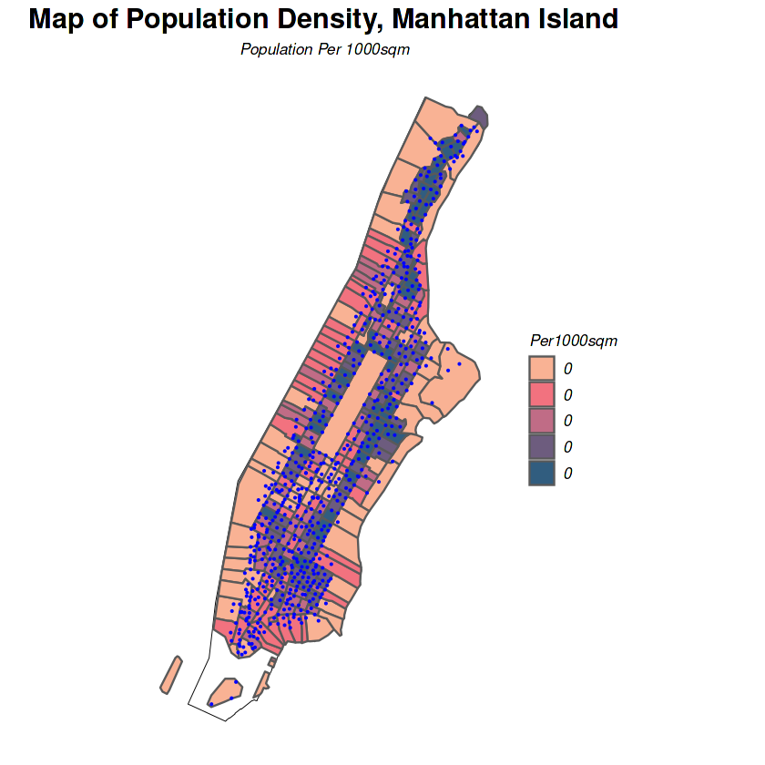
3.2 Census Data
Users of Citi bikes are citizens, therefore it is reasonable to assume that high population density may increase the need to use Citibikes.
Population data is added from Census data using census tract unit. Every bike dock is allocated population density data of its census tract.
census_api_key("", overwrite = TRUE)

nyCensus <- get_acs(geography = "tract",
variables = c("B01003_001E"),
year=2019, state="New York", county="New York",geometry = T, output="wide") %>%
st_transform(st_crs(NYCTracts)) %>%
rename(Census_TotalPop = B01003_001E) %>%
dplyr::select(-NAME,-starts_with("B")) %>%
mutate(Census_areasqm = as.numeric(st_area(.)),
Census_PopDensity = Census_TotalPop/Census_areasqm) %>%
dplyr::select(-Census_TotalPop,-Census_areasqm)%>%
replace(is.na(.),0)

nyTracts <- nyCensus %>%
as.data.frame() %>%
distinct(GEOID, .keep_all = TRUE) %>%
select(GEOID, geometry) %>%
st_sf

ggplot()+
geom_sf(data=st_union(NYCTracts),color="black",size=0.2,fill = "transparent")+
geom_sf(data=nyCensus,aes(fill=q5(Census_PopDensity)))+
geom_sf(data=ride_station,color="blue", size = 0.1)+
scale_fill_manual(values = palette5,
          labels = qBr(nyCensus, "Census_PopDensity"),
          name = "Per1000sqm")+
labs(title = "Map of Population Density, Manhattan Island",
subtitle = "Population Per 1000sqm")+
mapTheme()
3.4 Weather Features
Weather is an important to deteremine whether one is likely to bike or not. Does rain/precipitation affect ridership during rush hour?
NYC weather data is used to summarize, temperature, wind speed and precipitation on an hourly basis and plot the results over our study period.
weather.Data <- riem_measures(station = "NYC", date_start = "2022-04-15",
                  date_end = "2022-07-01")
weather.Panel <- weather.Data %>%
mutate_if(is.character,
list(~replace(as.character(.), is.na(.), "0"))) %>%
replace(is.na(.), 0) %>%
mutate(interval_hour = ymd_h(substr(valid, 1, 13))) %>%
mutate(week = week(interval_hour),
dotw = wday(interval_hour, label=TRUE)) %>%
filter(week %in% c(18:22))%>%
group_by(interval_hour, week, dotw) %>%
summarize(Temperature = max(tmpf),
Precipitation = sum(p01i),
Wind_Speed = max(sknt)) %>%
mutate(Temperature = ifelse(Temperature == 0, 42, Temperature)) %>%
replace(is.na(.), 0)
4. Exploratory Data Analysis
We begin by exploring the weather trends during our study period
grid.arrange(
ggplot(weather.Panel, aes(interval_hour, Precipitation)) +
geom_line(color = palette1_main, size = 0.5) +
labs(x = "", title = "Weather Data - Manhattan Island - NYC - Week 18 - Week 22 2022") +
plotTheme(),
ggplot(weather.Panel, aes(interval_hour, Wind_Speed)) +
geom_line(color = palette1_main, size = 0.3) +
labs(x = "", title = "" ) +
plotTheme(),
ggplot(weather.Panel, aes(interval_hour, Temperature)) +
geom_line(color = palette1_main, size = 0.6) +
labs(x = "Time", title = "") +
plotTheme()
)
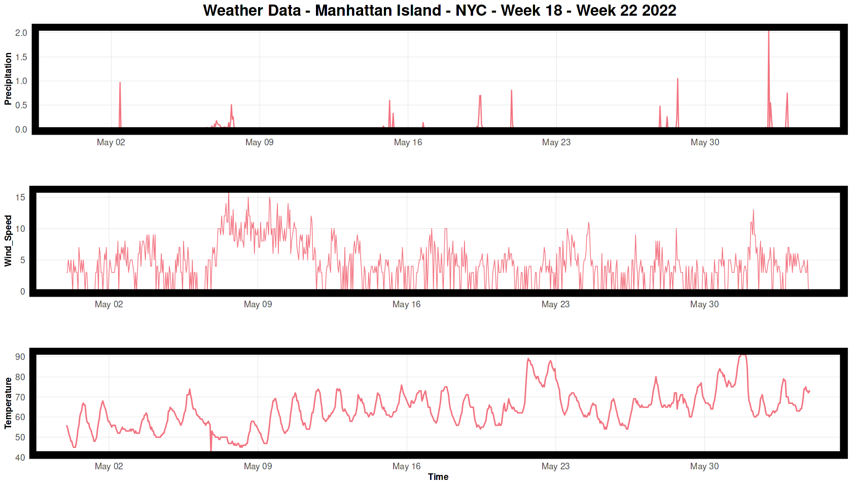
As you can see there was not much precipitation during the study months. Wind Speed has a spike in the second week, while temperature was gradually increasing over in the weeks.
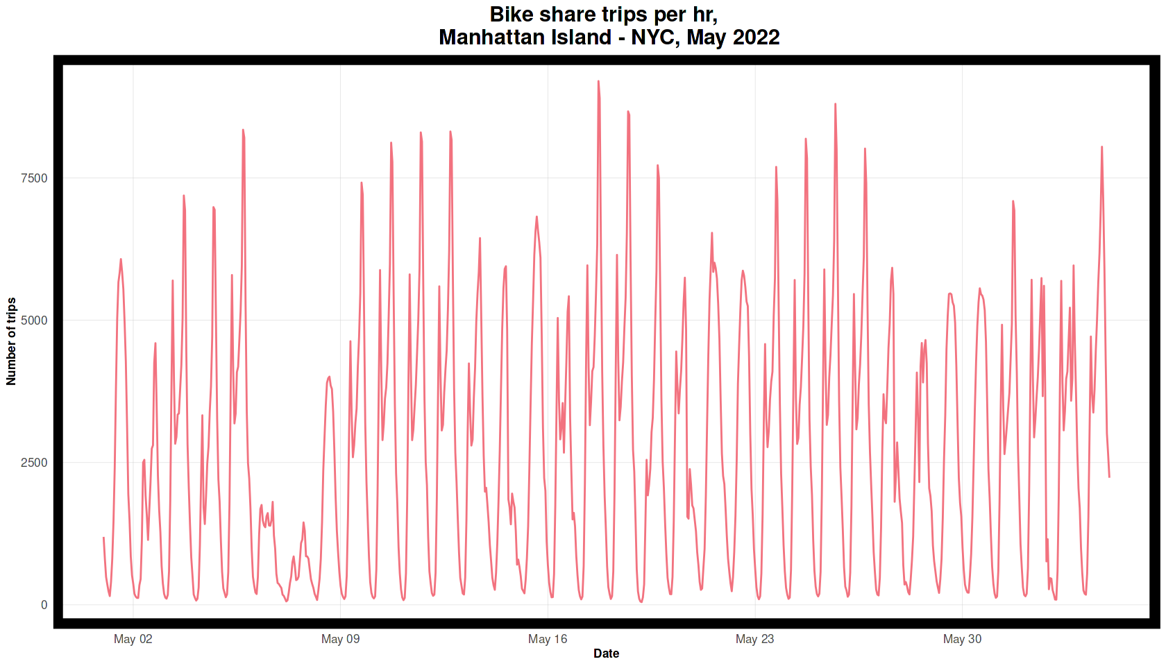
We take a look at the number of day trips during our study period -- there is clearly a daily periodicity and there are lull periods on the weekends.
nyBike_census <- nyBike_census %>%
mutate(interval_hour = floor_date(ymd_hms(started_at), unit = "hour"),
interval15 = floor_date(ymd_hms(started_at), unit = "15 mins"),
week = week(interval_hour),
dotw = wday(interval_hour, label = TRUE)) %>%
filter(week %in% c(18:22))

ggplot(nyBike_census %>% group_by(interval_hour) %>%
tally()) +
geom_line(aes(x = interval_hour, y =n), color = palette1_main, size = 0.6) +
labs(title = "Bike share trips per hr, \n Manhattan Island - NYC, May 2022",
x = "Date", y = "Number of trips") +
plotTheme()
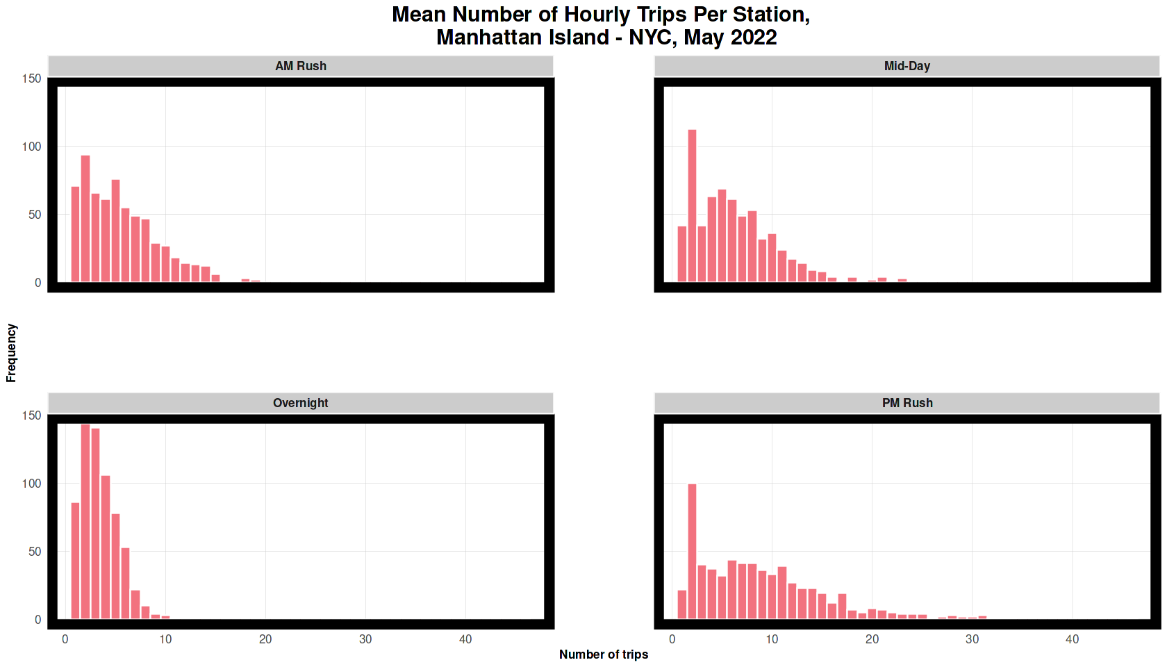
The plot below shows the mean number of hourly trips which is high during the morning and evening rush.
# mean number of hourly trips

nyBike_census %>%
mutate(time_of_day = case_when(hour(interval_hour) < 7 | hour(interval_hour) > 18 ~ "Overnight",
                    hour(interval_hour) >= 7 & hour(interval_hour) < 10 ~"AM Rush",
                    hour(interval_hour) >= 10 & hour(interval_hour) < 15 ~ "Mid-Day",
                    hour(interval_hour) >= 15 & hour(interval_hour) <= 18 ~ "PM Rush")) %>%
group_by(interval_hour, start_station_name, time_of_day) %>%
tally() %>%
group_by(start_station_name, time_of_day) %>%
summarize(mean_trips = mean(n)) %>%
ggplot() +
geom_histogram(aes(mean_trips), binwidth = 1, colour = "white", fill = palette1_main) +
labs(title = "Mean Number of Hourly Trips Per Station, \n Manhattan Island - NYC, May 2022", x = "Number of trips", y = "Frequency") +
facet_wrap(~time_of_day) +
plotTheme()
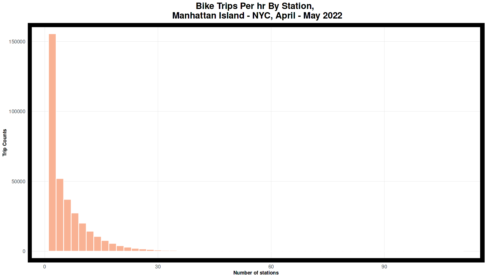
ggplot(nyBike_census %>%
group_by(interval_hour, start_station_name) %>%
tally()) +
geom_histogram(aes(n), binwidth = 2, colour = "white", fill = palette1_assist) +
labs(title = "Bike Trips Per hr By Station, \n Manhattan Island - NYC, April - May 2022",
x = "Number of stations", y = "Trip Counts") +
plotTheme()
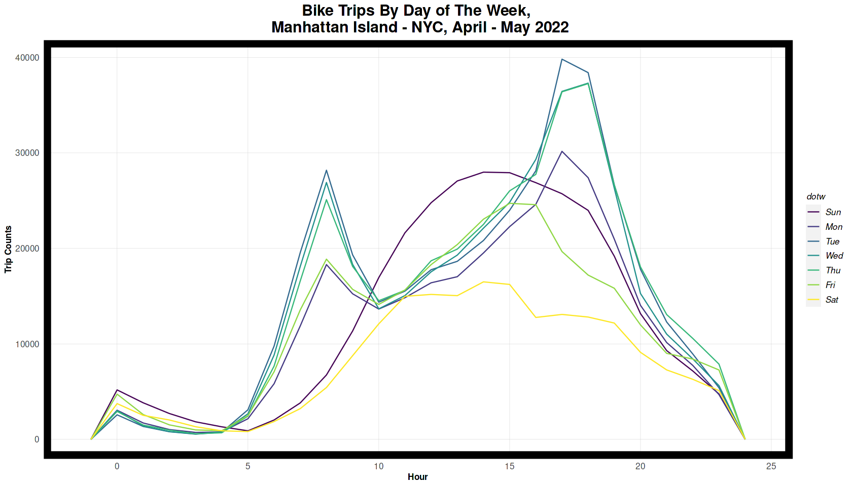
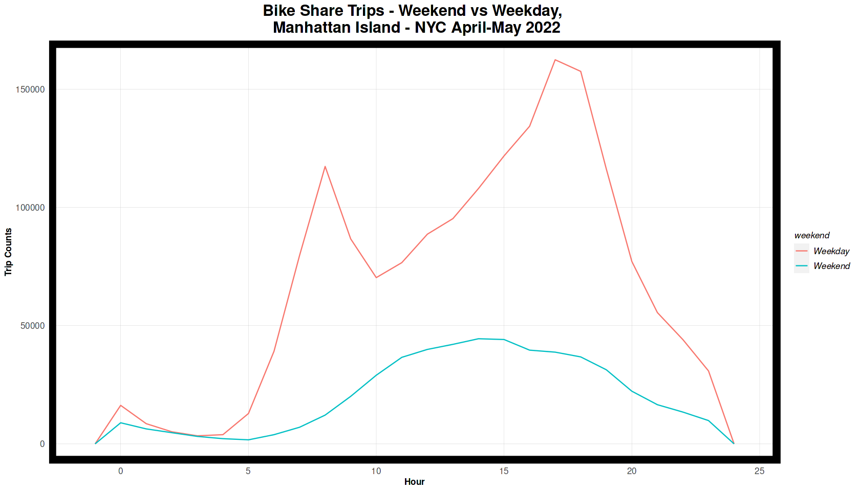
The plot below shows that most bike trips are during the weekday, with spikes in the morning and evening rush hours. During the weekends spikes are in the mid-morning and afternoon.
ggplot(nyBike_census %>% mutate(hour = hour(started_at))) +
geom_freqpoly(aes(hour, color = dotw), binwidth = 1) +
labs(title = "Bike Trips By Day of The Week, \n Manhattan Island - NYC, April - May 2022",
x = "Hour", y = "Trip Counts") +
plotTheme()
ggplot(nyBike_census %>% mutate(hour = hour(started_at),
                  weekend = ifelse(dotw %in% c("Sun", "Sat"), "Weekend", "Weekday"))) +
geom_freqpoly(aes(hour, color = weekend), binwidth = 1) +
labs(title = "Bike Share Trips - Weekend vs Weekday, \n Manhattan Island - NYC April-May 2022",
x = "Hour", y = "Trip Counts") +
plotTheme()
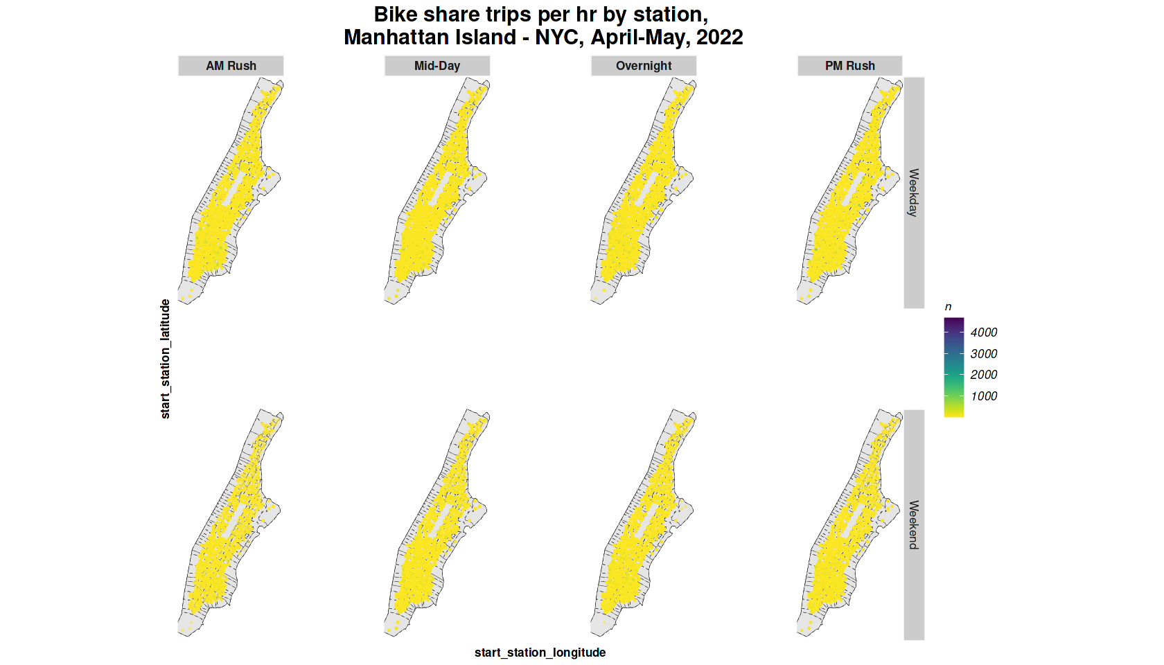
ggplot() +
geom_sf(data = st_union(NYCTracts), colour = "black", size = 0.1) +
geom_sf(data = NYCTracts, color = "black", size = 0.1, linetype = "dashed", fill = "transparent") +
geom_point(data = nyBike_census %>%
mutate(hour = hour(started_at),
        weekend = ifelse(dotw %in% c("Sun", "Sat"), "Weekend", "Weekday"),
        time_of_day = case_when(hour(interval_hour) < 7 | hour(interval_hour) > 18 ~ "Overnight",
                                hour(interval_hour) >= 7 & hour(interval_hour) < 10 ~ "AM Rush",
                                hour(interval_hour) >= 10 & hour(interval_hour) < 15 ~ "Mid-Day",
                                hour(interval_hour) >= 15 & hour(interval_hour) <= 18 ~ "PM Rush"))%>%
group_by(start_station_id, start_station_latitude, start_station_longitude, weekend, time_of_day) %>%
tally(),
aes(x=start_station_longitude, y = start_station_latitude, color = n),
fill = "transparent", alpha = 0.4, size = 0.3)+
scale_colour_viridis(direction = -1, discrete = FALSE, option = "D")+
ylim(min(nyBike_census$start_station_latitude), max(nyBike_census$start_station_latitude))+
xlim(min(nyBike_census$start_station_longitude), max(nyBike_census$start_station_longitude))+
facet_grid(weekend ~ time_of_day)+
labs(title="Bike share trips per hr by station,\n Manhattan Island - NYC, April-May, 2022")+
mapTheme()
4.1 Space Time Series
We create a time-series panel which basically is a unique combination of station id to the hour and day. This is done in order to create a data set where each time period in the study is represented by a row.
So if a station did not have any trips originating from it at a given hour, we still need a zero in that spot in the panel.
length(unique(nyBike_census$interval_hour)) * length(unique(nyBike_census$start_station_id))
529584
study.panel <- expand.grid(interval_hour = unique(nyBike_census$interval_hour),
              start_station_id = unique(nyBike_census$start_station_id)) %>%
left_join(., nyBike_census %>%
select(start_station_id, start_station_name, Origin.Tract, start_station_longitude, start_station_latitude) %>%
distinct() %>%
group_by(start_station_id) %>%
slice(1))

nrow(study.panel)
529584
trip.panel <- nyBike_census %>%
mutate(Trip_Counter = 1) %>%
right_join(study.panel) %>%
group_by(interval_hour, start_station_id, start_station_name, Origin.Tract, start_station_longitude, start_station_latitude) %>%
summarize(Trip_Count = sum(Trip_Counter, na.rm = T)) %>%
left_join(weather.Panel) %>%
ungroup() %>%
filter(is.na(start_station_id) == FALSE) %>%
mutate(week = week(interval_hour),
dotw = wday(interval_hour, label = TRUE),
Origin.Tract = as.character(Origin.Tract)) %>%
filter(is.na(Origin.Tract) == FALSE)

trip.Panel <- left_join(trip.panel, nyCensus %>%
as.data.frame() %>%
select(-geometry), by = c("Origin.Tract" = "GEOID"))
5. Feature Engineering
5.1 Time Lags
As seen in the exploratory analysis that morning and evening rush makes a difference in the demand for bikes. We creare time lags in our feature engineering that will give us additional information about the demand.
trip.Panel <- trip.Panel %>%
arrange(start_station_id, interval_hour) %>%
mutate(lagHour = dplyr::lag(Trip_Count, 1),
lag2Hours = dplyr::lag(Trip_Count,2),
lag3Hours = dplyr::lag(Trip_Count,3),
lag4Hours = dplyr::lag(Trip_Count,4),
lag12Hours = dplyr::lag(Trip_Count,12),
lag1day = dplyr::lag(Trip_Count,24)) %>%
mutate(day = yday(interval_hour))

trip.Panel <- trip.Panel %>%
mutate(X = start_station_longitude, Y = start_station_latitude) %>%
st_as_sf(coords = c("X", "Y"), crs = 4326, agr = "constant") %>%
st_transform(st_crs(NYCTracts))

as.data.frame(trip.Panel) %>%
group_by(interval_hour) %>%
summarise_at(vars(starts_with("lag"), "Trip_Count"), mean, na.rm = TRUE) %>%
gather(Variable, Value, -interval_hour, -Trip_Count) %>%
mutate(Variable = factor(Variable, levels = c("lagHour","lag2Hours","lag3Hours","lag4Hours",
                                  "lag12Hours","lag1day"))) %>%
group_by(Variable) %>%
summarize(correlation = round(cor(Value, Trip_Count), 2))
| Variable | Correlation |
|---|---|
| fct | dbl |
| lagHour | 0.90 |
| lag2Hours | 0.71 |
| lag3Hours | 0.51 |
| lag4Hours | 0.33 |
| lag12Hours | -0.54 |
| lag1day | 0.79 |
There is a Pearson's R of 0.90 for the lagHour. As mentioned in the intro, the demand pattern for the hour is similar to that of last year and todays pattern is similar to that of yesterday and tomorrow.
5.2 Exposure Features
Apartments, Parks & Population
Here we look at two exposure features -- apartments and parks. Reasonable assumptions are that the number of population will be larger id the number of apartments and parks are larger. More population means more chance of using bike share system.
q0 <- opq(bbox = c(-74.025203,40.699282,-73.901210,40.881792))

get_osm_1 <- function(bbox, key, value, geom, crs){
object <- add_osm_feature(opq = bbox, key = key, value = value) %>%
osmdata_sf(.)
geom_name <- paste("osm_", geom, sep = "")
object.sf <- st_geometry(object[[geom_name]]) %>%
st_transform(crs) %>%
st_sf() %>%
cbind(., object[[geom_name]][[key]]) %>%
rename(NAME = "object..geom_name....key..")
return (object.sf)
}

apartments = get_osm_1(q0, "building", "apartments", "points", st_crs(NYCTracts))
apartments_select <- st_intersects(st_union(NYCTracts) %>%
                      st_sf(), apartments)
apartments2 <- apartments_select[[1]]
apartments3 <- apartments[apartments2,]

park = get_osm_1(q0, "leisure", "park", "polygons", st_crs(NYCTracts)) %>%
st_centroid()
park_select <- st_intersects(st_union(NYCTracts) %>%
                st_sf(), park)
park2 <- park_select[[1]]
park3 <- park[park2,]
grid.arrange(ncol = 2,
ggplot() +
    geom_sf(data=st_union(NYCTracts), color = "black", size = 1, fill = "transparent") +
    geom_sf(data = NYCTracts, color = "black", size = 0.3, linetype = "dashed", fill = "transparent") +
    geom_sf(data = park3, size = 0.4, color = palette1_main) +
    labs(title = "Map of Parks Manhattan Island - NYC",
        subtitle = "Red dots are parks") +
    mapTheme(),
ggplot() +
    geom_sf(data=st_union(NYCTracts),color="black",size=1,fill = "transparent")+
    geom_sf(data=NYCTracts,color="black",size=0.3,linetype ="dashed",fill = "transparent")+
    geom_sf(data=apartments3,size=0.3,color=palette1_main)+
    labs(title = "Map of Apartments Manhattan Island - NYC",
        subtitle = "Red dots are apartments") +
    mapTheme()
)
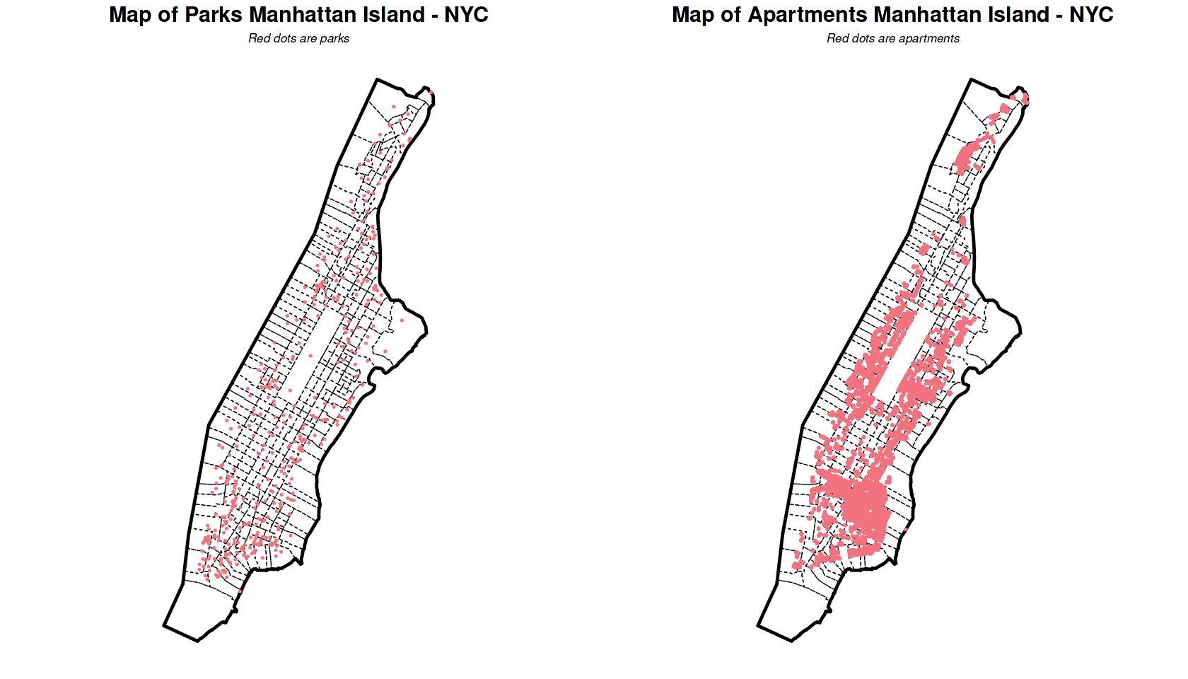
The above plot, we can see a relatively evenly distribution of parks, and a south-concentrated distribution of apartments.
The distance to the 5 nearest parks and apartments is calculated and added into every station. The transformed 5 apartments distance data into every station.
trip.Panel_coord = st_coordinates(trip.Panel)
park3_coord = park3 %>% dplyr::select(geometry) %>% st_coordinates
apartments3_coord = apartments3 %>% dplyr::select(geometry) %>% st_coordinates

trip.Panel <- trip.Panel %>%
mutate(park_nn5 = nn_function(trip.Panel_coord, park3_coord, 5),
apartment_nn5 = nn_function(trip.Panel_coord, st_coordinates(apartments3), 5))

trip.Panel <- trip.Panel %>%
mutate(apartment_nn5 = as.numeric(apartment_nn5),
trans_apartment_nn5 = log(1+sqrt(trip.Panel[['apartment_nn5']]))) %>%
replace(is.na(.), 0)
6. Linear Regressions
We split our data into a training and test set. Training on 3 weeks of data, weeks 18-20, and testing on the following 2 weeks 21-22. If the time/space is generalizable, it can be used to project into the near future.
trip.Train <- filter(trip.Panel, week < 21)
trip.Test <- filter(trip.Panel, week >= 21)
In this section, five different Linear regressions are estimated with different fixed effects:
- reg1 focuses on just time, including additional features
- reg2 focuses on just space fixed effects, including additional features
- reg3 focuses on time and space fixed effects, including additional features
- reg4 focuses on time, space fixed effects, time lag features and additional features
- reg5 adds time, space fixed effects, time lag features, nearest distance to apartments and parks and additional features
6.1 Predictions for test dataset
I ran out of available memory. My computer memory at the time of this project was 16GB RAM. I will revisit this project soon.
# trip.Test.weekNest <-
#   as.data.frame(trip.Test) %>%
#   nest(-week)

# trip.Test.weekNest

# model_pred <- function(dat, fit){
#   pred <- predict(fit, newdata = dat)}

# week_predictions <-
#   trip.Test.weekNest %>%
#   mutate(ATime_FE = map(.x = data, fit = reg1, .f = model_pred)
#          BSpace_FE = map(.x = data, fit = reg2, .f = model_pred),
#          CTime_Space_FE = map(.x = data, fit = reg3, .f = model_pred),
#          DTime_Space_FE_timeLags = map(.x = data, fit = reg4, .f = model_pred),
#          ETime_Space_FE_timeLags_Features = map(.x = data, fit = reg5, .f = model_pred)
#         ) %>%
#   gather(Regression, Prediction, -data, -week) %>%
#   mutate(Observed = map(data, pull, Trip_Count),
#          Absolute_Error = map2(Observed, Prediction,  ~ abs(.x - .y)),
#          MAE = map_dbl(Absolute_Error, mean, na.rm = TRUE),
#          sd_AE = map_dbl(Absolute_Error, sd, na.rm = TRUE))

# week_predictions